Here are the test data series. And here are the functions that created them, in case you want to start from scratch... Indeed, here is the script that created all the Matlab plots on this page.
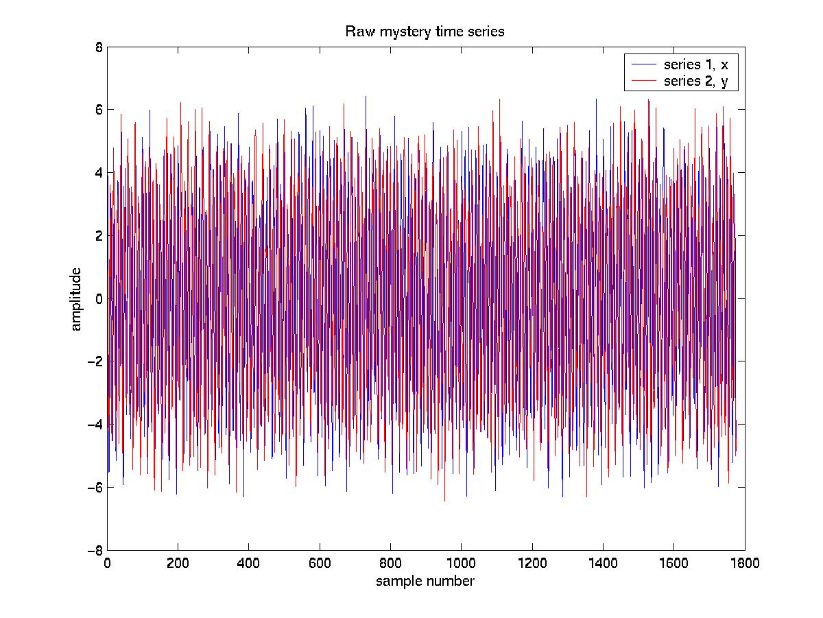
Here is a plot of the raw data:
By examining just a few oscillations of the 2 time series (below) we can make some initial estimates of the values for the periods and phase lags (a good thing to do with natural series, too).
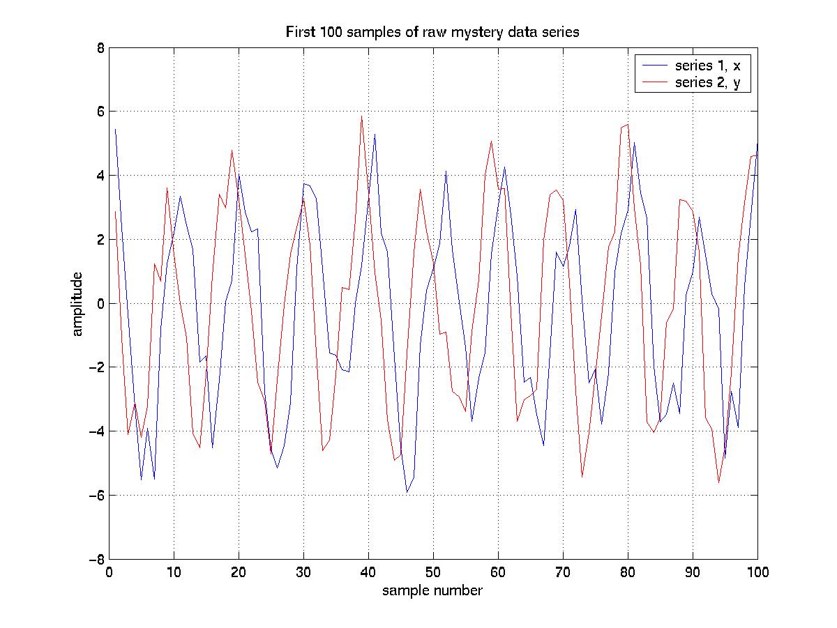
It looks like series 1 (blue, and hereafter called x) has a period of about 10 data samples, or 10 hours if we assume the sampling rate was 1 per hour. Series 2 (red, and hereafter called y) appears to have the same period, but lead x by about 2 hours. So x should have a phase lag (relative to y) of 2 hours, or -(2/10)*360=-72 degrees.
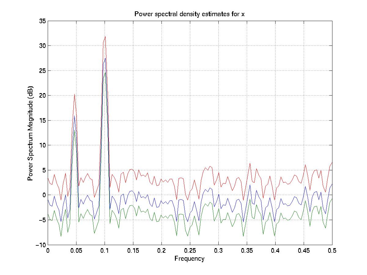
The next 3 figures show the results of 3 psd or csd commands (in which the arguments are: the data series (each 1024 samples long); the number of samples in each subseries of to transform; the sampling frequency; the Hanning window full width; and the amount of overlap in the subseries):
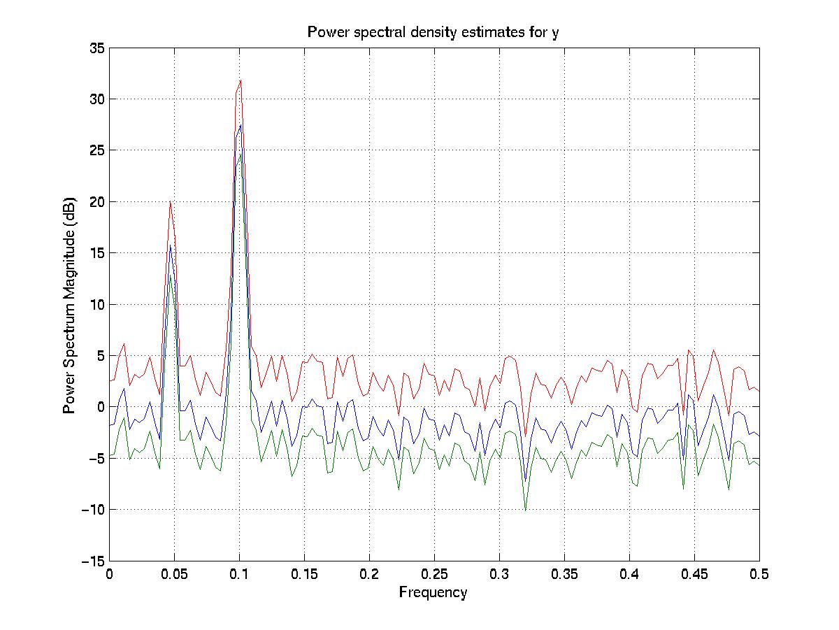
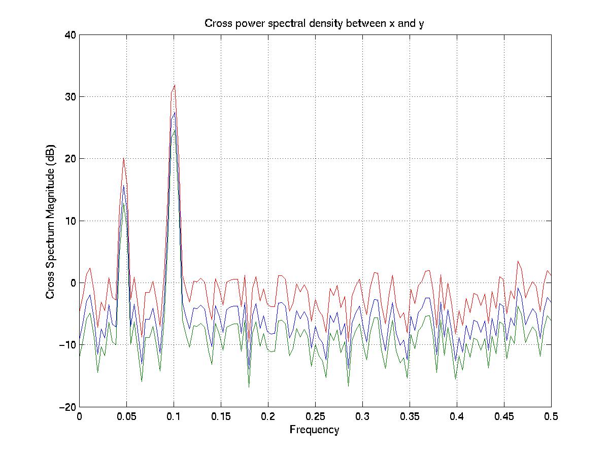
[gxx,gxxc,f]=psd(x,256,1,256,0,.95);
gyy=psd(y,256,1,256,0,.95);
gxy=csd(x,y,256,1,256,0,.95);
coh= abs(gxy).^2 ./ (gxx.*gyy);
phase= atan2(-imag(gxy),real(gxy)) * 180/pi;
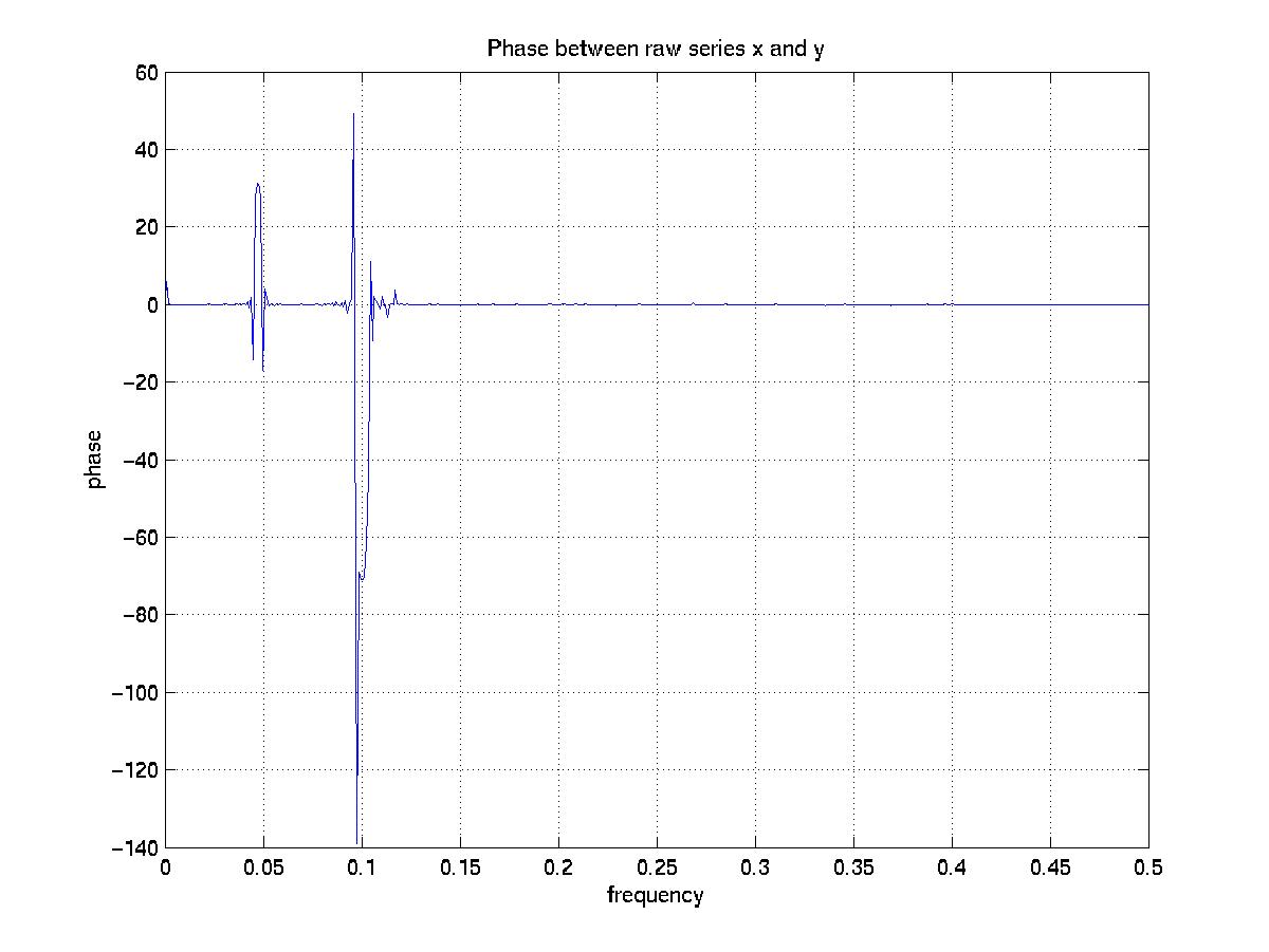
The plots of coh and phase as functions of frequency (f) are plotted next:
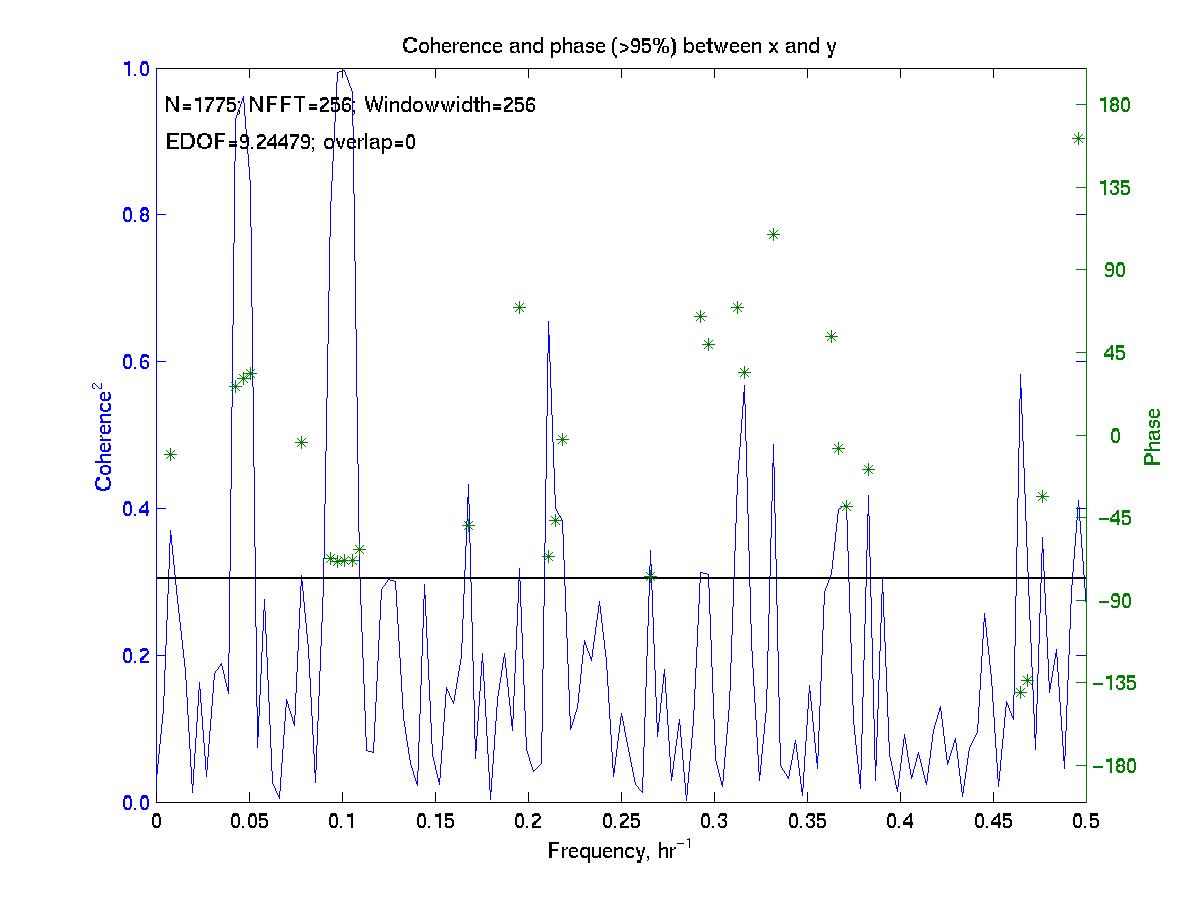
The coherence squared has 2 prominent peaks that rise above the 95% confidence level (horizontal black line): one at a frequency corresponding to a 10 hour period and another with slightly lower coherence near 0.045 cph (21 hour period). Further averaging in the time or frequency domain will reduce the number of spurious peaks (above 95% confidence level) at higher frequencies.
The phase of the 2 most coherent peaks are -70 degrees (x lags y) at the 10 hr period and +30 degrees (x leads y) at a period near 22 hrs.
A slightly different averaging scheme led to the following plot from Bill Lavelle (note that the random numbers were different from those in the above plots...)
The FFT approach
For comparison, we can try to calculate the power spectra and cross spectrum via smaller steps (that are hard to monitor within the psd and csd commands).
The Matlab commands (to detrend, window, and tranform the series)
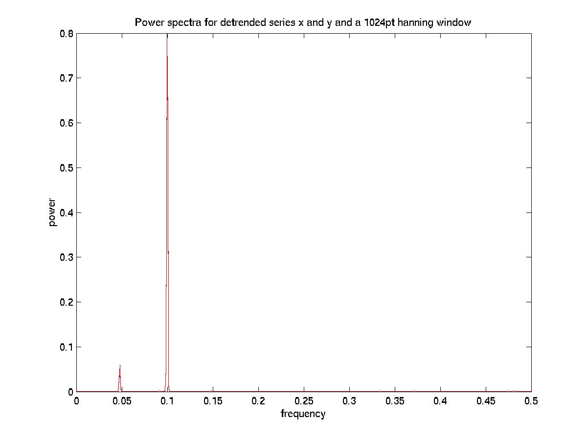
n=1024;
f=(1/2)*(0:512)/512;
fftdhx=fft(detrend(x).*hanning(n),n);
fftdhy=fft(detrend(y).*hanning(n),n);
% Note discrepancy in following psd calculation:
% McDuff (http://www2.ocean.washington.edu/oc540/lec01-12/matlab.html) divides by n^2
% Emery and Thomson divide by n*dt, where dt=sampling period, and then rescale the transforms by root(8/3)
%   to compensate for energy lost during windowing
psdhx=fftdhx.*conj(fftdhx)/n^2;
psdhy=fftdhy.*conj(fftdhy)/n^2;
plot(f,psdhx(1:1+n/2),'b');
plot(f,psdhy(1:1+n/2),'r')
yield the following raw power spectra (which are virtually identical for x (blue) and y(red)) and show peaks at frequencies of 0.45 and 0.1 (periods of 10 and 22 "hours"):
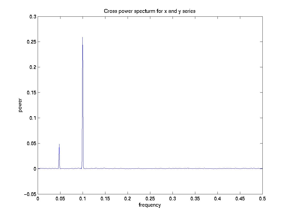
Ignoring the McDuff/Thomson discrepancy for now, I compute the cross power spectral density estimate in an analogous fashion (dividing by n^2):
csdxy=conj(fftdhx).*fftdhy/n^2;
plot(f,real(csdxy(1:1+n/2)),'b')
This generates a cross spectrum that has peaks at the same frequencies:
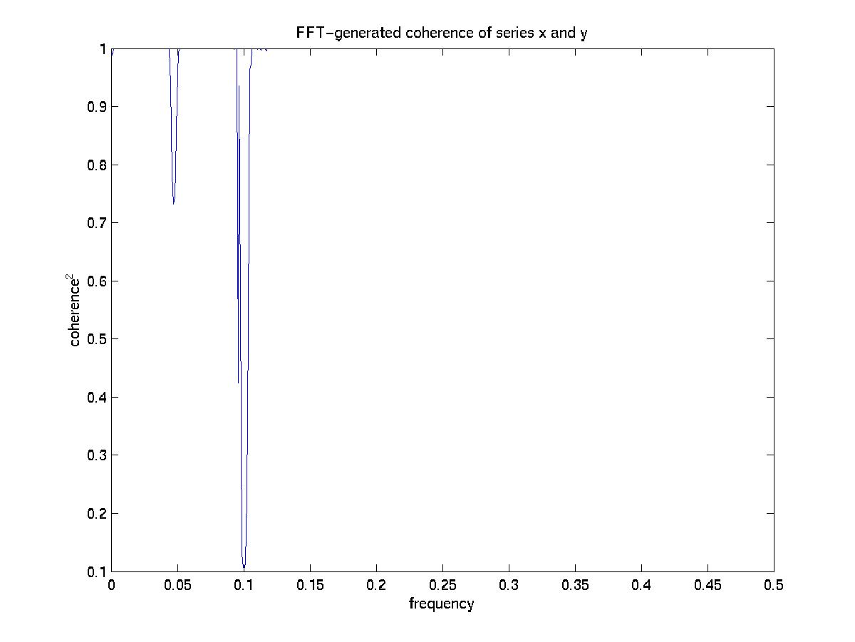
Finally, I calculate coherence and phase as before
% Note Matlab runs into some precision problems in the calculation of fftcoh
% when the very small complex coefficients of csdxy are squared
% I've commented out the emery/thomson formula, and (incorrectly?) used:
%fftcoh= abs(csdxy).^2 ./ (psdhx.*psdhy);
fftcoh= real(csdxy).^2 ./ (psdhx.*psdhy);
fftphase= atan2(-real(csdxy),imag(csdxy)) * 180/pi;
plot(f,fftcoh(1:1+n/2),'b');
plot(f,fftphase(1:1+n/2),'r');
Plots of fftcoh and fftphase versus f look like:
Again, it's easier to read a plot of 1-fftcoh:

The series appear to be coherent at 0.045 and 0.1 frequencies, or 21.5 and 10 "hour" periods. The final plot suggests that at these frequencies, the phase separation is near +30 and -70 degrees, respectively (though it might be clarified significantly through some averaging).
In summary, the coherence and phase diagrams generated with the 2 techniques look pretty consistent; the psd/csd curves look like averaged versions of the raw curves. One remaining points of confusion is why the coherence function is equal to 1 for most frequencies, rather than 0.