Matlab xcorr and coh analysis of N/S Flow Mow currents

load_wasp2161;
load_50mm;

The script cross_corr_curr.m does the following:

1. Calculates along/across axis components of velocity (called v and u)
2. Gets maximum temporal overlap between the 2 series
3. Linearly interpolates both series to the same 1hr interval time base
4. Detrends and plots both series
5. Calculates and plots auto and cross correlation functions

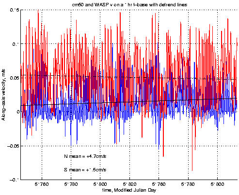
Here is an ascii file of the 2 resulting v time series. The 3 columns contain: (1) modified julian day (time centered on observed hour); (2) the along-axis component of hourly mean velocity at the N meter (2161m depth, 16m above sea floor); (3) the along-axis component of hourly mean velocity at the S meter (2168m depth, 50mab).

Here are the 2 v time series and their trend lines. The red curve is the N data, while the blue curve is the S data. The Flow Mow cruise and heat flux observations occurred between MJD 51760-51776.

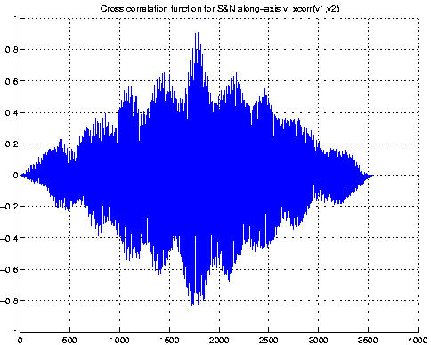
Now the Matlab function xcorr(v1,v2) calculates the cross-correlation function (v1=south data, v2=north data). The function (plotted below) has a domain of 3549 points and a maximum amplitude at point 1787. 3548/2=1774, so the cross correlation peak is (1787-1774=) 13 points to the right of the domain center. If you take the median of all values greater than 0.8, you get 1775, suggesting that the N meter leads the S meter by 1 hour, rather than 13 hours. I wonder how you decide what the exact peak is in order to specify the phase lag?

Next: PSD and CSD approach to coh and phase