MATLAB Time Series Example

In this example we will use a synthetic data set. To create our synthetic data we will make our unit of time 1000 years = 1 ky and sample a 500,000 year record in 2 ky increments. We first create a vector containing the times:

t=0:2:500;

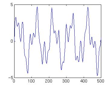
We want this record to have multiple periodic components. To mimic the orbital forcing of the Earth's climate, we create a vector d, of the same length as vector t and with components that have periods of 100 ky, 41 ky and 21 ky, weighted 2.5:1.5:1, then plot it

echo off
axis ([0 500 -5 +8])
echo on

d=2.5*sin(2*pi*t/100)+1.5*sin(2*pi*t/41)+1*sin(2*pi*t/21);
plot(t,d)

()

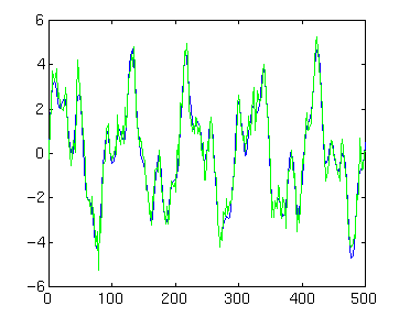
We add some normally distributed random noise to the record to create a new record dn, and plot it on the same graph:

dn=d+0.5*randn(size(d));
hold
plot(t,dn,'g')

()

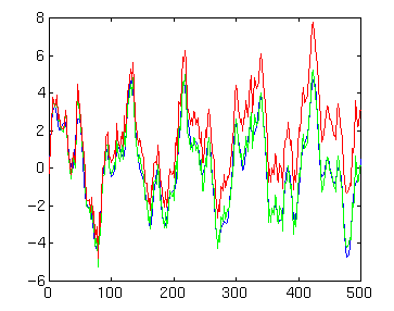
We also add a long term trend to create a third record dnt, and again plot it on the same graph

dnt=dn+3*t/500;
plot(t,dnt,'r')

()

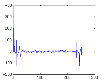
Our time series has 251 elements. To improve computation efficiency we will pad it with zeros and extended it to 256 elements (a power of 2). This is done implicitly with the fft command. Then taking the Fourier transform and plotting its real part:

DNT=fft(dnt,256);
hold off
plot(real(DNT))

()

By convention, the transform has elements equally spaced in frequency, with the first element corresponding to f=0, then up to the Nyquist frequency at the middle of the record, then the negative frequencies from large to small in the remaining elements. The negative frequencies contain redundant information so we want to look only at the positive frequencies. These frequencies are evenly spaced within the Nyquist interval (for our 2 ky sampling interval the Nyquist frequency is 1/4 ky):

f=0.25*(0:128)/128;

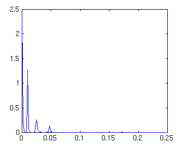
The power spectrum of the record is estimated as:

PNT=DNT .* conj(DNT)/(256*256);

hold off
plot (f,PNT(1:129))

()

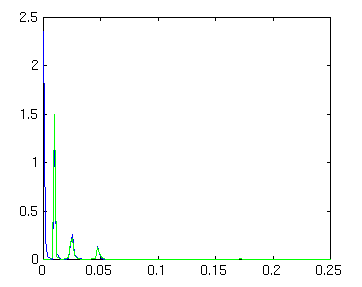
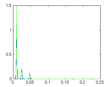
We easily see the peaks at frequencies of about .01, .025 and .05 per ky with the power in approximate proportion to the amplitude squared (25:9:4 or approximately 6:2:1). Notice the power present as the frequency goes to 0 corresponding to the long term (d.c.) trend. This can be removed by detrending the data which for us is equivalent to working with the dn record. Applying the same steps:

DN=fft(dn,256);
PN=DN .* conj(DN)/(256*256);
hold
plot (f,PN(1:129),'g')

()

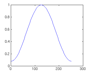
We see that the low frequency contamination is removed. We will work with detrended dn record from now on. Next we will apply a window-- a Hamming window in particular

z=hamming(251);
plot(z)

()

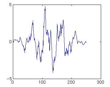
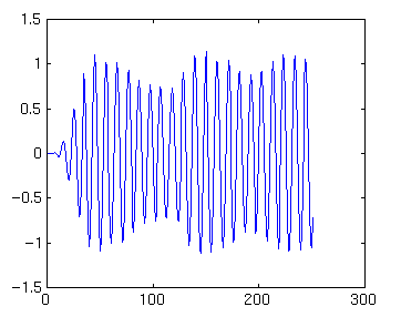
Multiplying the dn record by this window:

dnz=dn .* z';
plot(dnz)

We now take the power spectra of this windowed time series (PNZ) and compare to the situation with no window (PN)

DNZ=fft(dnz,256);
PNZ=DNZ .* conj(DNZ)/(256*sum(z));
plot (f,PNZ(1:129))
hold
plot (f,PN(1:129),'g')

We are also interested in details of the time series itself. To extract parts of record, say the 21 ky band, we need bandpass filter to let through frequencies between say .04 to .06/ky. Here we use a Butterworth filter, one of the many possibilities:

[b,a]=butter(5,[.04/.25 .06/.25]);
plot (filter(b,a,dn))

()

We find ~500/21=24 cycles of approximately the right amplitude (1) once we are 5 cycles into series. (There are ways of minimizing these end effects).

We also wanted to look at spectral characteristics of autocorrelated data:

dna=xcorr(dn);
plot (dna)

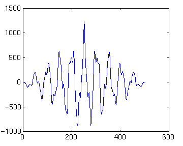Zero lag is plotted in the middle of diagram, with negative lag to the left and positive to the right. The plot is symmetric because the record is compared to itself. We find the power spectra of the autocorrelated data:

DNA=fft(dna,512);
PNA=DNA .* conj(DNA)/(512*512);
f2=.25*(0:256)/256;
plot(f2,PNA(1:257,:))

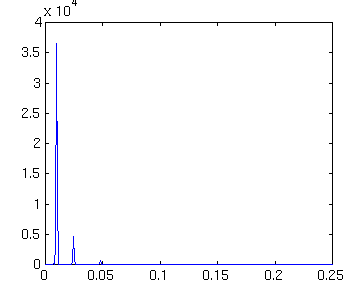We find the same spectral character working with the autocorrelation, the difference being that the power is a measure of the variance due to that periodic component, i.e., most of the variance is explained by the 100 ky period.