Sediment Accumulation

Deposition and Accumulation of Marine Sediments

The sediment record that accumulates below the sea floor is rarely identical with the sediment that is initially deposited by oceanographic processes (Figure SA-1). Only where bottom currents are weak and the oxygen value at the sea floor is virtually zero (thereby inhibiting bioturbation) are relatively pristine records preserved. These conditions are found at such locations as the Santa Barbara Basin off southern California, Saanich Inlet, north of Victoria, B.C., Guymas Basin in the Gulf of California, Orca Basin in the Gulf of Mexico, the Black Sea, and the Cariaco Trench off Venezuela. These sites have been studied intensely to unravel the highest frequency changes in oceanographic and depositional conditions.

Figure SA-1. Processes that intervene to change the characteristics of freshly deposited sediment prior to its incorporation into the geologic record.

Bioturbation mixes the new sediment with older material, thereby acting as a low pass filter of the record of depositional change. In addition, if the incoming sediment is poorly sorted, bioturbation can separate the coarse particles from the fine ones, which can be concentrated at the sea floor (armoring). Erosion, whether physical, physical plus biological (which can result in the removal of material at very low bottom current velocities), or chemical, all create gaps or distortions of the preserved record. The change in elevation of the sea floor over time can be described in terms of the bulk density of the surface sediment, the flux of incoming material, and lateral transport.

Equn. SA-1:

Where the del term is positive (lateral convergence), sedimentation is enhanced by lateral transport (as is the case in the drift deposits of the North Atlantic, for example). In contrast, divergence (negative del term) results in erosion.

The rate of deposition and the processes that modify freshly accumulated sediment can be unraveled by the use of radioactive isotopes. The use of ¹⁴C to interpret the Holocene dissolution of equatorial Pacific carbonate deposits will be discussed in a future lecture. Other useful radiotracers are members of the U and Th decay series. In unweathered minerals, the daughter isotopes of the decay of the primordial radioactive isotopes ²³⁸U and ²³²Th are in equilibrium with the parent (i.e. the absolute decay rate of all isotopes in a series is the same). During the surface geochemical cycle, however, the daughters are separated from the parents and begin to decay as independent species, each with its characteristic half life. In the case of ²³⁸U (Figure SA-2), daughters such as ²³⁴Th (t1/2 = 24 days), ²³⁰Th (75,000 years), ²²⁶Ra (1,622 years) and ²¹⁰Pb (21.4 years) have been used to interpret sediment deposition.

Figure SA-2. Chain of isotopes produced by the radioactive decay of ²³⁸U. Downward shifts in the table result from alpha decays (loss of a He nucleus), shift up and to the right result from beta decays (loss of a nuclear electron). Half lives of radioactive isotopes are shown in years (Y), days, (D), minutes (M) and seconds (S).

For ²³²Th (Figure SA-3), the daughters ²²⁸Th (1.9 years), ²²⁴Ra (3.6 days) and ²¹²Pb (10.6 hours) have been used in the same way.

Figure SA-3. Chain of isotopes produced by the radioactive decay of ²³²Th. Symbols as Figure SA-2.

In radioactive decay, the number of atoms decaying depends only on the number present,

i.e. - dN/dt = lambda * N, where lambda is the decay constant. If the number of atoms of a radionuclide at time zero is N_o, then the number N_t at time t is:

Equn. SA-2:

Where C is any measure of concentration of the nuclide. Since the accumulation rate (A) is dz/dt, A is given by:

Equn. SA-3:

Where, in this case, the depth interval z is measured from the sea floor. This relation ignores the effect of bioturbation, which mixes fresh and decayed sediment. For a steady state,

Equn. SA-4:

Where the first term describes bioturbation, the second burial, and the third, radioactive decay. This yields:

Equn. SA-5:

Which, by comparison with Equn. SA-3, shows that the accumulation rate will be overestimated if bioturbation is not taken into account. The two unknowns, A and D can be determined by measuring two isotopes with different half lives. Ideally, one is chosen with a half life close to the characteristic time for bioturbation and the other with a half life equivalent to deposition over several bioturbated layer depths. The limited selection of available radionuclides does not always make this possible, however!

Identifying Sediment Sources

Most sediments are derived from two or more independent sources. One of the challenges facing sedimentologists and geochemists is to unravel these sources, both because of the paleoenvironmental information they carry, and because mobile elements will interact differently with the different sediment components. Individual minerals differ in their crystal form, lattice spacing, and location of elements within the crystal lattice. As a result, each mineral lattice diffracts X-rays slightly differently. Such differences are used to identify the minerals present in a sample, and to estimate the abundance of each. Unfortunately, this technique rarely fully characterizes a sample because of the presence of amorphous or poorly diffracting phases, and because appropriate standards for many naturally occurring minerals (particularly those which are very fine grained) are not available. As a result, much effort has been devoted to developing strategies to partition elemental composition data into source components. This is a classic inverse problem, where the compositions of the sources are rarely known with certainty.

Mixing models. For the case of two end members, A and B, containing a% and b% of some element, the proportion of A in an unknown sample containing x% of the element is (b-x)/(b-a) (assuming that x lies between a and b). In general, however, more than two end members, a,b,c, ..., are involved, their exact compositions are uncertain or variable, and there are analytical uncertainties associates with a,b,c, ...,x.

A number of different techniques have been used to address this problem. They include:

Factor analysis. This technique, which is a form of objective analysis, will be discussed in much more detail in the lecture on proxies, where it will be used to reduce abundance data for a large number of microfossils in a sample to a more manageable number of statistically independent groupings or factors. Elemental abundances can be substituted for species abundances to yield statistically independent geochemical factors.

The selection of the appropriate number of factors is subjective and is usually guided by geographic or temporal coherence in the distribution of each factor. A serious limitation of the method is that unless the sample set includes members the compositions of which are close to those of the end members, the compositions of the factors will bear little relation to real source materials. Thus, the proportions of each factor making up each sample will be difficult to interpret in physical terms. Various mathematical strategies have been applied to solve this problem, but none are satisfactory in all cases.

Component stripping. If the concentration of an element is much higher in one end member than in all the others, it can be used to estimate the proportion of that end member in all the samples. That proportion, together with the known concentration of other elements in that end member can be used to remove the contribution of that end member to each element in the sample, i.e.

For end member A, consisting of A(a)%. A(b)%, A(c)%, ... of elements a, b, c, ... respectively, where A(a) >> B(a), C(a), ... (the concentration of a in all other end members), the proportion of A in sample X is X(a) / A(a). A's contribution to elements b, c, d ... in X is (X(a)/A(a)) *A(b), ... and the unexplained part of b, c, ... is :

Equn. SA-6:

The process can be repeated if the concentration of a second element is much greater in B (or A and B) than in any of the remaining end members, and so on.

This approach works quite well in an area such as the East Pacific Rise west of South America. There, the sediment consists largely of detritus from South America that is rich in Al relative to other components, hydrothermal plume precipitates from the Rise crest that are rich in Fe relative to non-detritus components, biogenic material from the overlying water column that is rich in Zn relative to the remaining component, and authigenic material precipitated slowly from seawater. The stripping technique yields proportions that are comparable to those from more sophisticated interpretive techniques.

The method's weaknesses are its requirement for strong elemental differentiation between end members (which is unlikely in the case of two detrital end members, for example), its inability to convey any sense of the uncertainty in the calculated contributions of the end members, and the propagation of errors resulting from several successive subtractions like that of Equn. SA-6. In addition, it requires that all the end members and their compositions be known.

Linear programming. The requirement that elements be strongly partitioned between end members makes the analysis easier, but is not necessary if the number of elements exceeds the number of end members. In this case, for four end members (as above) and n elements, there are n equations of the form:

Equn. SA-7:

where i is the ith element, D,H,B, and A are subscripts for pure detrital, hydrothermal, biogenic, and authigenic ratios, respectively, and D_Al, H_Fe, B_Si, and A_Ni are the (unknown) amounts of detrital Al, hydrothermal Fe, biogenic Si, and authigenic Ni in the sample, respectively, and R_i is the residual or "error". To solve, we rearrange to:

Equn. SA-8:

For n elements, this yields n+4 equations. A conventional least squares analysis usually results in negative contributions for one or more of the end members. Linear programming allows for restrictions on the solution. For sediment partitioning, end member contributions are restricted to positive values or zero, and the sum of R_i over all elements is minimized. D_Al can be converted to total detritus if the Al content of detritus is known. The same for the other end-member elements, allowing the weight fraction of each end member to be determined.

The weakness of this method is its requirement that end member compositions be known, and that R_i be minimized (if one or more end members are overlooked, for example, the true R may be large). In addition, trace element concentrations have to be scaled so that the major elements do not dominate the solution to the problem.

Total inversion. The total inversion method, developed for solving geophysical problems (A.Tarantola and B.Valette, 1982, Rev. Geophysica and Space Physics, v. 20, pp. 219-232) does not distinguish strongly between knowns (the elemental analyses) and unknowns (end member compositions and abundances). All are considered "data" and are treated as input variables with specified uncertainties. This allows variable analytical uncertainties as well as uncertainties about end member compositions to be factored into the solution. During the inversion, the magnitude of the uncertainties control the adjustment allowed for each variable. The method differs most significantly from the others in allowing the end member compositions to vary from sample to sample, which is probably more geologically realistic than the assumption of fixed end member compositions. Figure SA-4 shows the end member compositional data and their uncertainties used as input to a total inversion model of sediment composition of a North Pacific red clay core spanning the last 70 million years.

Figure SA-4. Concentrations and uncertainties in concentrations of elements in eight end members used to partition North Pacific red clay sediments in core GPC-3 (Figure SA-5).

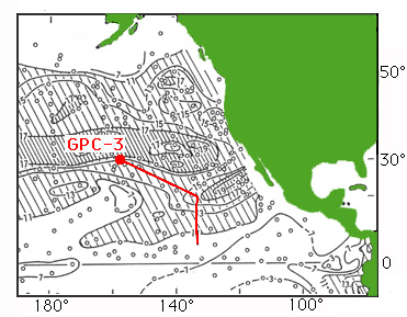
Figure SA-5. Location of Core GPC-3 showing its displacement relative to the hot spot reference frame during the past 65 Ma (due to absolute drift of the Pacific Plate) and to present-day quartz abundances in surface sediments.

The inverse model was able to simplify concentration data for 39 elements in 324 samples (Figure SA-6,7) into eight end members that varied coherently through time in a geologically and oceanographically reasonable way (Figure SA-8). Such modelling allows sediment budgets to be generated in a reproducible and transparent way and to be modified easily in the light of new information.

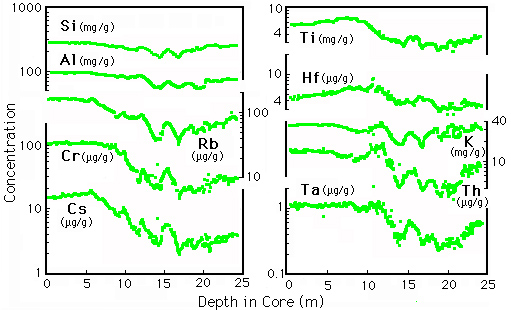
Figure SA-6. Profiles of elemental abundances versus depth in core GPC-3. These elements are predominantly of terrigenous origin. The variations result from movement of the core site and flux variations from multiple sources.

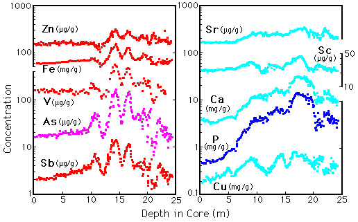
Figure SA-7. Profiles of elemental abundances versus depth in core GPC-3. These elements include substantial hydrothermal (left) and biogenic (right) contributions.. The variations result from movement of the core site and flux variations from multiple sources.

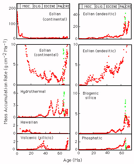
Figure SA-8. Variations in the fluxes of seven end members to core GPC-3 during the past 70 My, estimated by total inversion of the core sample and end member compositional data. The green dots indicate samples from the Cretaceous-Tertiary boundary layer, where the model fit to the data is less satisfactory due to the presence of extraterrestrial material (characterized by high Ir concentrations) associated with the K-T meteorite impact.