This lecture begins a module of lectures concerned with the processes involved in heat and mass transfer through the ocean crust. These are processes that shape the ocean basins, imparting its topography and morphology and serving as a major conduit for transfer of materials from the Earth's interior. In this group of lectures, we address the question of how heat is transported as the lithosphere forms and evolves on scales ranging from tectonic plate, to melt generation and migration into the crust, to transfer of heat from hot rock to convecting fluid.

Conduction

Eq 3-1:

(conductive heat flux, q) = - (thermal conductivity, k) x (temperature gradient, dT/dz)

The negative sign reflects that heat is transported in the direction of lower temperature. For a historical discussion of Fourier's Law and its influence on the description of other physical systems, see (44). In dimensional terms:

Dimensions for Heat Transfer Quantities

	recent literature	older literature
flux	W m	cal cms
thermal conductivity	W m°C	cal cms°C
gradient	°C m	°C m

The pratical unit from older literature is the HFU (heat flow unit). 1 HFU (heat flow unit) = 41.9 mW m = 1 µcal cms

The global average conductive heat flow is about 2 HFU.

The thermal conductivity (or equivalently the specific thermal conductivity, (also called the thermal diffusivity) which includes the density and heat capacity of a material) varies considerably, over about four orders of magnitude in various solid materials:

Thermal Conductivities of Common Materials

	k [W m°C]	=k/(C) [ms]
	thermal conductivity	specific thermal conductivity or thermal diffusivity
solid silver	420
fiber glass	0.04
surficial ocean sediment	0.9	2x10
basaltic rock	2.9	7.7x10
upper mantle	3.1	8x10

Using observations of the conductive heat flow we can estimate the temperature increase with depth into the oceanic lithosphere. At 100 My crustal age the heat flow is ~1.1 HFU = 46 mW m, so:

Eq 3-2:q=-k(dT/dz)

Eq 3-3:46 x 10 W m = 3.1 W m°C (dT/dz)

Eq 3-4:(dT/dz) = 15 x 10 °C m

Thus, at 100 km depth, T ~1500 °C. (This is an overestimate, as even after 100 My, the lithosphere is continuing to cool and so the profile is not strictly linear.)

This approach is reversed in order to make heat flow measurements: the temperature gradient is measured with a probe consisting of a number of thermistors which is inserted into sediment; the thermal conductivity is measured (by measuring the response after a thermal perturbation) or estimated from other data; the product yields the heat flow.

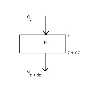
To make use of Fourier's Law we need to establish a thermal balance for a small volume element. In one-dimension, balance the fluxes of heat through the two surfaces and the internal production of heat per unit volume, H, determine the temperature change in an interval of time dt:

Figure 3-1

Conservation of heat requires that:

Eq 3-5:

Rearranging equation 3-5 and taking to limits:

Eq 3-6:

Is Internal Production of Heat Important Within the Lithosphere?

Well away from the ridge axis where the time rate of change becomes small, it becomes appropriate to consider the steady-state characteristics of equation 3-6. The goal is to examine whether the internal production of heat, H has a significant influence on the temperature distribution.

At steady state:

Eq 3-7:

Equation 3-7 is solved by integrating twice to find:

Eq 3-8:

The two constants of integration are found by specifying the temperature at the sediment surface:

Eq 3-9:

and the surface heat flow

Eq 3-10:

Combining equations 3-8, 3-9 and 3-10, we find:

Eq 3-11:

If H=0, the temperature increases linearly with depth. For positive internal production of heat, there is a negative deviation from this linear trend which grows as z squared. (The deviation is negative because of the boundary conditions we have chosen; as H increases more of the surface heat flux is derived from internal production of heat and less from the flux of heat from below). In the case of the lithosphere, is this deviation important? Because the elements U, Th and K are partitioned into the liquid as the mantle melts, considering the radiogenic production of heat in the basaltic crustal layer represents a worst case (i.e., the mantle must have a lower content of U, Th, and K). This production is 7.8x10 W m. At 6 km depth, for surface heat flow of 45 mW m and with this value of H the temperature deviation is 0.97°C from the value without internal production, 93°C. We conclude that we can generally neglect internal production of heat.

Thus for application to conductive heat loss from the lithosphere we neglect H and equation 3-6 becomes:

Eq 3-12:

Conductive Plate Model--Boundary Layer Approach

Eq 3-13:

Imagine that at the axis of spreading that material is held at the temperature of melting, in other words an appropriate initial condition is that at all depths:

Eq 3-14:

(While we will not develop it explicitly, 'temperature' here means 'potential temperature'). For now also imagine that the Earth is infinitely thick, i.e., the geometry is that of an infinite half space and so at great depth:

Eq 3-15:

Finally the upper surface will be will be held at the temperature of the deep ocean:

Eq 3-16:

Omitting the details of solution, we find that:

Eq 3-17:

(note the k inside the root operator should be kappa) We can use equation 3-17 to calculate the temperature field of an evolving lithosphere.

While there are some problems evident in the model (specifically 1) the temperature of the seafloor at the ridge axis is not T_m and 2) the thickness of the lithosphere does not grow without limit), it is appears to be reasonable from a qualitative standpoint and so we will use it as a starting point for considering the relationships among heat flow, topography and crustal age.

Conductive Heat Flow versus Age

By taking the derivative of equation 3-17 to obtain an expression for dT/dz evaluated at z=0 and substituting into equation 3-2 we find that (details):

Eq 3-18:

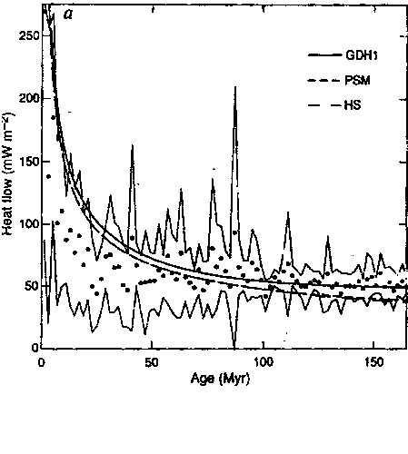
The heat flow predicted from the boundary layer model decreases with an inverse proportionality to the square root of age.

For now (we will later refine these parameters) we can estimate the relationship using a value of T of 1400 °C and the thermal conductivity data given in Table I:

Eq 3-19:

480 mW/m is ~12 HFU.

Conductive heat flow versus age, from (43)

HS is the infinite half space model, PSM is the original Parsons Sclater model, GDH1 is the more recent Stein and Stein fit to the global data set. (HS and PSM can only be distinguished on very old lithosphere)

Topography versus Age

Thermal contraction of the lithosphere increases its density and so isostatic adjustment will result in subsidence of old lithosphere as it ages. Consider this model:

Figure 4-1

If we compare the masses (we should actually consider the weights, but we will take the gravitational acceleration as constant) of the two columns A (at the rift axis) and B (at some arbitrary age), we can derive a relationship for the subsidence, w.

Mass of column A

Eq 4-1:

Mass of column B

Eq 4-2:

where w is the water depth below the ridge, z is the thickness of the lithosphere, and is density. The subscripts w, L and m denote water, lithosphere, and melted mantle (i.e., asthenopshere), respectively. Equating M and M and rearranging:

Eq 4-3:

The left term is positive, since the lithosphere is cooler and denser than the asthenopshere, and represents the effect of thermal contraction; the second term is negative and represents the effect of replacing denser mantle with lighter seawater as the seafloor subsides.

The specific volume, v, is a state variable v=v(T,P) and so a variation of v can be represented by:

Eq 4-4:

where is the isothermal compressibility and is the volumetric coefficient of thermal expansion. For an unconstrained material the pressure does not change when the temperature and volume change, i.e., dP=0, and:

Eq 4-5:

but

Eq 4-6:

Therefore the change in density associated with thermal contraction can be expressed, using plastic, uncooled mantle as a datum (the "M" subscript):

Eq 4-7:

The temperature distribution in the lithosphere is taken from the conductive boundary layer model for the plate (rewriting the solution in terms of erfc(x)=1-erf(x)):

Eq 4-8:

Substituting equations 4-7 and 33-8 into equation 33-3 and solving for w we find that:

Eq 4-9:

Because the error function complement term in the integral of equation 4-9 approaches zero at the base of the lithosphere, the upper limit of integration can be changed from z to infinity without introducing appreciable error. (This is equivalent to saying T-T approaches zero at the base of the lithosphere, see equation 4-7). With this change of limit and the variable substitutions:

Eq 4-10:

equation 4-16 becomes:

Eq 4-11:

With this substitution, the definite integral in equation 4-11 can be evaluated:

Eq 4-12:

so that:

Eq 4-13:

Since the depth to the seafloor is of the form:

Eq 4-14:

a depth age relationship can be expressed:

Eq 4-15:

We can make an estimate of w using a value of T of 1350 °C and the thermal conductivity data given in Table I:

Eq 4-16:

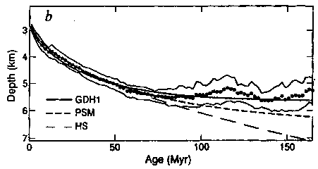
Seafloor topography versus age, from (43)

HS is the infinite half space model, PSM is the original Parsons Sclater model, GDH1 is the more recent Stein and Stein fit to the global data set.

Variants on Boundary Layer Model

Three refinements to the boundary layer approach have been considered in the literature and applied in variations combinations (see Parsons and Sclater(8) for references):

1. extending the model to two dimensions and explicitly considering the horizontal advection of heat by the plate:

   Eq 4-17:

2. With T(x=0)=T, the heat flux was unbounded at the axis of spreading. Refine the boundary condition at the ridge axis so that heat leaving the axis by conduction and advection matches the heat carried by injected material (i.e., apply a flux condition)

3. Establish a geometry for the model domain such that there is an asymptotic plate thickness and fix the temperature at that lower boundary.

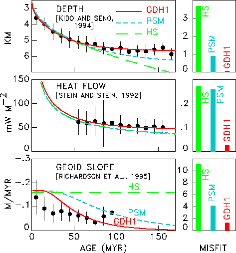
In the past decade, Stein and Stein (43) have undertaken a substantial effort to revisit various aspects of the plate model in order to take full advantage of the data sets that have been obtained since the early Parsons and Sclater work. More information is available at the Seth Stein page.

Material properties can be extracted from best fits of improved models (Parsons and Sclater, 8, Stein and Stein (43)):

Fits to Parameters of the Plate Model

	North Pacific (8)	North Atlantic (8)	Global (43)
asymptotic lithospheric thickness (km)	125	128	95
boundary temperature (°C)	1333	1365	1450
thermal expansion coefficient (°C)	3.3 x 10	3.1 x 10	3.1 x 10-5

The agreement is quite satisfying in that each of these three parameters can be related to other observations (the thickness of the lithosphere to seismic studies of upper mantle structure, the boundary temperature to laboratory observations and thermodynamic calculations of melting of mantle rock, the thermal expansion coefficient to studies of physical properties of mantle rock).