PLEISTOCENE GLACIAL CYCLES

What do we know about Pleistocene climate?

1. Numerous proxies show strong periodicities with periods of 23, 41, and 100 ky (Figure GC-3)

2. The amplitude of proxy peaks at periods of 23 and 41 ky can be explained by linear forcing by precession and tilt of the earth's axis (Figure GC-1, 2) as represented by the level of incoming radiation at 65º N.

Figure GC-1. Variations in the amplitude of ¹⁸O and radiation cycles

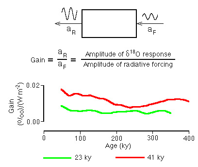
Figure GC-2. Gain in the precession and frequency bands as a function of time for the past 350-400 ky. The amplitude of incoming radiation at 65º N is used as forcing and the amplitude of the ¹⁸O signal in the same bands is used as response.

3. The significance and magnitude of phase relations between tilt (41 ky period) and proxies are ambiguous because both hemispheres are impacted identically. Because the same lags (due, presumably, to the same processes) also occur in the 23 ky (precession) band in which the radiation effects on the hemispheres are out of phase, however, the initial effects must originate in the northern hemisphere

Table 29-1. Response times relative to northern and southern forcing

	41 ky	23 ky
Relative to northern forcing	20-94 deg	30-158 deg
	2-11 ky	2-10 ky
Relative to southern forcing	20-94 deg	210-338 deg
	2-11 ky	13-22 ky

4. Phase lags between the spectra of different proxies and inferred radiative forcing yield consistent and physically reasonable sequences of oceanographic processes for each glacial-interglacial cycle (Figure 22-7).

An examination of 14 proxies (Figure GC-3) shows that 11 have similar phase relations in all three frequency bands. They can be separated into a group that leads ice volume (¹⁸O) and a group that lags ice volume.

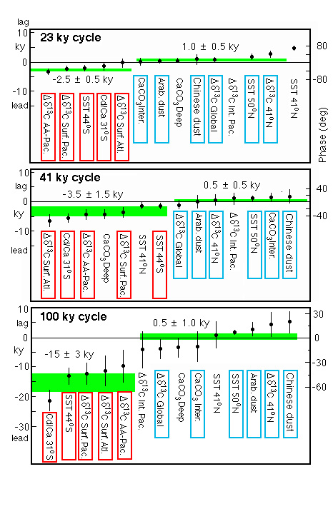
Figure GC-3. Mean lag times and phases for 14 climatic proxies relative to ¹⁸O at the Milankovitch orbital frequencies.

Proxies that lead ¹⁸O:

• Antarctic - Pacific ¹³C
• Surface - Deep Pacific ¹³C
• Surface - Deep Atlantic ¹³C
• Cd/Ca (i.e. PO4^-3) at 31º S in the South Atlantic
• Sea surface temperature at 44º S

All these proxies are related to the magnitude of the flux of NADW. All would be expected to respond rapidly to events in the Nordic Sea that increase or decrease the rate of formation of NADW.

Proxies that lag ¹⁸O:

• CaCO₃ dissolution at intermediate depths in the Caribbean
• Flux of dust to the Arabian Sea
• Rate of accumulation of Chinese loess
• Global ¹³C (changes in the mass of the terrestrial biosphere)
• Sea surface temperature at 50º N in the North Atlantic
• Proportion of NADW at 41º N in the eastern North Atlantic

All these proxies are responses to the build-up of significant northern hemisphere ice masses.

In terms of years, the average lag times for both the lead and lag groups are indistinguishable in the 23 ky and 41 ky bands, suggesting that the response mechanisms of the earth's climatic system to forcing are the same at these two frequencies. For the 100 ky band, the average lag is the same, whereas the lead time is about four times as long as for the other two frequencies.

5. Given the striking variations in the flux of NADW, a likely area for initial responses is the Nordic Sea, as defined by Imbrie et al. Because long proxy records suitable for spectral analysis do not exist for this area, the issue must be assessed in the time domain.

Figure GC-4 shows the relations of a number of processes during Termination 1, the conclusion of the last ice age. These events are well dated by ¹⁴C.

• The earliest event is the increase in early June incoming radiation at 65º N.

  This is followed by the initial retreat of the margins of the Laurentide ice sheet which appears to be in phase with the increase in ¹⁶O (i.e. decline in ¹⁸O) in the world ocean.

  This is closely followed by a spike of ¹⁸O depleted water in the Nordic Sea, which is attributed to the initiation of massive melting of the northern hemisphere ice sheets

  This is followed by accelerated retreat of the ice margin and rise in sea level.

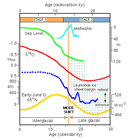
Figure GC-4. Evidence that northern hemisphere deglaciation at the end of the last ice age was a response to orbital forcing and that the earliest responses were in the northern Atlantic (Nordic Sea) region.

The frequency and time domain observations can be simulated by a simple mathematical model. For example, suppose there is a single forcing (incoming radiation) and a single response ( ¹⁸O) variable. Then for a system with a delay time d and a response time T, the phase delay at frequency f is given by:

= 2fd+arctan(2fT)

Since there are analogous phase delays in both the 23 and 41 ky bands, the two equations in two unknowns can be solved to yield d of about 1 ky and T of about 17 ky. Both are plausible, given the response times of the ocean and a large continental ice mass.

As discussed earlier, Imbrie et al. conclude that four climatic states are involved in the Pleistocene climatic cycles. They modify the simple mathematical model accordingly (Figure GC-5) to include a single delay time of 1 ky and three response times of 3, 5, and 0.5 ky.

Figure GC-5. Mathematical model of 23 and 41ky responses to radiative forcing at 65º N. Si are linear subsystems (components listed at top of figure) having either delays (d) or time constants (T).

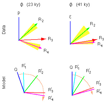
Figure GC-6. The phase clocks show the goodness of fit between the model of Figure GC-5 and data. Note that R1 is not sampled by the available time series, but is inferred from the time domain relationships.

After iteration, the fit between models and data is reasonable, particularly if the date of maximum 65º N radiation is shifted from mid-June to early June or late May.

The 100 ky problem

The simple model developed for the linearly forced precession and tilt frequency bands cannot be applied directly to the eccentricity (100 ky) band. Some of the issues:

1. The forcing generated by eccentricity variations is too weak (Figure GC-7) to produce the responses observed in the terrestrial climate proxies.

Figure GC-7. Partitioning of incoming 65º N June radiation and ¹⁸O (ice volume) record into precession, tilt, and eccentricity bands. Note the striking discrepancy between the amplitudes of the radiation and ice volume time series in the 100 ky band.

2. The eccentricity record has power at periods of both 100 and 400 ky, whereas the ice volume record only shows 100 ky power. At 100 ky, there is fair agreement between the two signals (Figure GC-8).

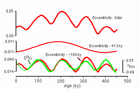
Figure GC-8. Eccentricity showing 100 ky and 400 ky cycles during the past 500 ky. After removing the 400 ky cycle, the amplitudes of the eccentricity and 100 ky ¹⁸O records are quite similar.

3. The time evolution of the spectra of the two parameters over the past 2 my (Figure GC-9) is very different. The amplitude of the 100 ky peak in the eccentricity spectrum is decreasing whereas the amplitude of the same peak in the ice volume record is increasing.

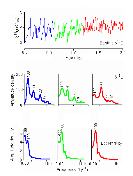
Figure GC-9. Benthic ¹⁸O record for the past 2 my showing the increasing importance of the 100 ky frequency band. In contrast, the amplitude of the 100 ky eccentricity signal declines over the same period.

4. The sequence of proxy phase leads and lags relative to ice volume is the same for the 100 ky band as for the other two, but the time delay between the early response group and ice volume (¹⁸O) is 15 ky rather than about 3 ky (Figure GC-3).

5. Subtraction of the 23 and 41 ky contributions to the total ¹⁸O record (Figure GC-10) leaves a residual that is very similar to the 100 ky band-pass filtered record.

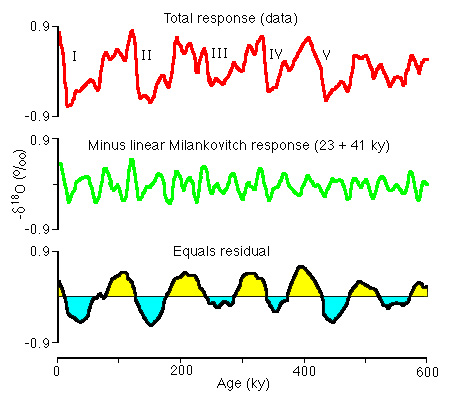
Figure GC-10. Residual ¹⁸O signal after stripping the linear responses to precession and tilt.

6. Models of icecap development without 100 ky forcing nevertheless develop free oscillations with periods in the 70-130 ky range.

In a recent paper, Shackleton (Science , v. 289, p. 1897, 2000) has compared ¹⁸O and CO₂ in trapped air in the Vostok ice core with deep-sea ¹⁸O records. By independently tuning the ice and oceanic records to the Milankovitch tilt and precession cycles, he concludes that in the100 ky band, maximum NH summer radiation, deep water temperature, antarctic ice surface temperature (based on D/H ratio), and atmospheric CO₂ are in phase (with 95% confidence), whereas ice volume lags by about 15 ky (Figure GC-11). This result throws no extra light on the link between eccentricity and the correlated proxy changes, however.

Figure GC-11. Amplitude, coherence, and phase spectra for deep-sea temperature (A), and ice volume (B) from deep sea sediments and for D/H (C) and CO₂ (D) from the Vostok ice core relative to an eccentricity(e)-tilt(t)-precession(p) record that assigns roughly equal variance to each component and with the phase of midsummer Northern Hemisphere insolation. The solid line is the amplitude spectrum, the shaded area the coherence spectrum, and the phase spectrum (with 95% confidence limits) uses the convention that a positive angle is a phase lag (from Shackleton, op cit.)

From their observations, Imbrie et al. drew the following conclusions

1. Linear forcing by variations in incoming radiation due to eccentricity is not possible.

2. The similarity of the phase lag groupings of proxies in all three frequency bands suggests that the climate system operates similarly at all three periods, although with a longer delay between early responses and ice volume at 100 ky.

3. The similarity of the ice volume and eccentricity records in the 100 ky band is compatible with a resonance phenomenon in which "pacing" of the ice volume record by eccentricity phase locks the two records.

The model developed for the 23 and 41 ky responses (Figure GC-5) works for the 100 ky record (Figure GC-12), as long as the ice volume time constant is increased from 5 ky to 15 ky.

Figure GC-12. Imbrie et al. model for the 100 ky climate cycle compared to the 23/41 ky model (Figure GC-5). Note the longer response time for S3.

This led Imbrie et al. to suggest that the 100 ky climatic signal results from non-linear amplification of the incoming radiation signal (Figure GC-13) once an internal critical threshold is exceeded.

Figure GC-13. Conceptual model for climate where the response is linear until a threshold is crossed, after which the response is disproportionately amplified.

They suggest that this threshold is set by feedbacks (albedo, atmospheric circulation) that develop when northern hemisphere icecaps exceed a critical size which interferes with the re-establishment of the Nordic heat pump by radiation increases at the higher frequencies.

The system is paced by eccentricity because of its influence on the amplitude of the incoming radiation signal in the 23 ky band. The key appears to lie in the extension of the icecaps on to isostatically depressed continental shelves as the ice masses approach maximum size. Once this happens, even a small sea level rise (due to peak radiation at the precession frequency, for example) results in destabilization of the ice caps with rapid melting that leads to further destabilization. Such rapid collapses produce the "Terminations" which are such a prominent feature of the late Pleistocene ice volume record.

The detailed sequence of atmospheric, ice cap, and oceanographic events during the last two terminations (Figure GC-14, 15) is compatible with this concept.

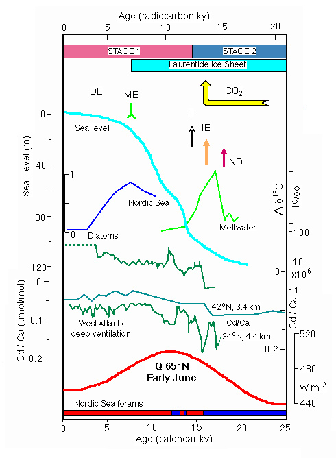
Figure GC-14. Sequence of events in the Nordic Sea - North Atlantic region during Termination 1 (the transition from the last ice age to the present interglacial). ND=major Nordic deglaciation event, IE=increased exchange of Atlantic water, T=maximum temperature rise, ME=maximum exchenge of Atlantic water, DE=decreased exchange of Atlantic water, meltwater = Greenland Sea - global ¹⁸O.

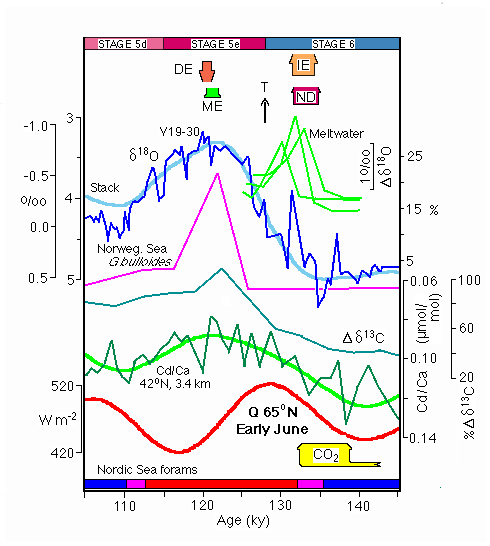
Figure GC-15. Sequence of events in the Nordic Sea - North Atlantic region during Termination 2 (the transition from the penultimate ice age to the last interglacial). Abbreviations as Figure GC-14. Note the age uncertainties (in CO₂, ND, IE, purple sections in Nordic Sea forams) relative to Termination 1, which is well dated by ¹⁴C.

Recently, Maureen Raymo and her colleagues (e.g. Ridgwell et al ., 1999, Paleoceanography, v. 14, no. 4, pp.437-440) have suggested that low 65º N summer radiation peaks that occur every fourth or fifth precessional cycle lead to a build-up of "excess" ice on the icecaps, followed by rapid deglaciation during the next precessional peak. Time series analysis of a mixed 4+5 precessional cycle yields a 100ky spectral peak that resembles the SPECMAP ¹⁸O peak. Because the low summer radiation precession peaks result from modulation by eccentricity, such a 100 ky spectral peak will be in phase with eccentricity.

Still unexplained is the geologically rapid evolution of the 100 ky spectral peak in ¹⁸O records compared to the 23 and particularly the 41 ky records which have been relatively stable for the past two million years (Figure GC-9).

Hypotheses to explain the increasing importance of the 100 ky cycle focus on modifications to the ice covered regions by a succession of glaciations. Examples include:

• the gradual stripping of the regolith (surface soil and weathered rock layer) which is thought to act as a lubricant that prevents the build-up of very thick ice, and
• downcutting of the continental shelf by ice streams so that the toes of the streams are well below modern sea level and are, therefore, vulnerable to collapse as a result of small rises in sea level due to radiation increases at 65º N resulting from Milankovitch forcing.