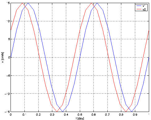
t=0:1/24/1;
vo=15; cm/s
omega=2*3.14159/(12/24)
lag=1/24;
v1=vo*sin(omega*t);
v2=vo*sin(omega*(t+lag));
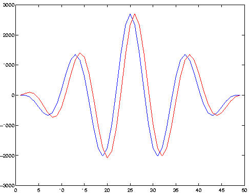
Now we use the Matlab function xcorr(v1,v2) to calculate the cross-correlation function.
In the figure below, the blue curve is xcorr(v1,v1) [no lag], while the red curve is xcorr(v1,v2) [1hr lag]. Note that the red curve has a peak at sample #26, while the blue peaks at sample #25. This means that a peak at more positive sample # indicates that the second function leads, not lags, the first. So maybe this should be called a phase-lead plot, or negative phase-lag plot?
Now on to a comparison of N and S current meter data...