A Model of Glacial-Interglacial Cycles

Phasing of Proxies

An examination of 14 proxies (Figure 1) shows that 11 have similar phase relations in all three frequency bands. They can be separated into a group that leads ice volume (¹⁸O) and a group that lags ice volume.

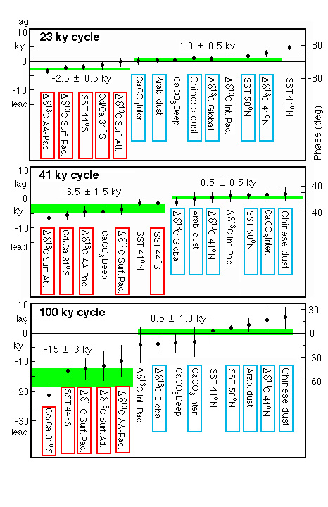
Figure 1. Mean lag times and phases for 14 climatic proxies relative to ¹⁸O at the Milankovitch orbital frequencies.

The average lag times for both the lead and lag groups are indistinguishable in the 23 ky and 41 ky bands, suggesting that the response mechanisms of the earth's climatic system to forcing are the same at these two frequencies. For the 100 ky band, the average lag is the same, whereas the lead time is about four times as long as for the other two frequencies.

• Antarctic - Pacific delta ¹³C
• Surface - Deep Pacific delta ¹³C
• Surface - Deep Atlantic delta ¹³C
• Cd/Ca (i.e. PO4) at 31 S in the South Atlantic
• Sea surface temperature at 44 S

All these proxies are related to the magnitude of the flux of NADW. All would be expected to respond rapidly to events in the Nordic Sea that increase or decrease the rate of formation of NADW.

The proxies that lag ¹⁸O are:

• CaCO₃ dissolution at intermediate depths in the Caribbean
• Flux of dust to the Arabian Sea
• Rate of accumulation of Chinese loess
• Global delta ¹³C (changes in the mass of the terrestrial biosphere)
• Sea surface temperature at 50 N in the North Atlantic
• Proportion of NADW at 41 N in the eastern North Atlantic

All these proxies are responses to the build-up of significant northern hemisphere ice masses.

This timing can be illustrated in a time series from the Nordic Seas. Figure 2 shows the relationship of a number of processes during Termination 1, the conclusion of the last ice age. These events are well dated by 14-C.

• The earliest event is the increase in early June incoming radiation at 65 N.
• This is followed by the initial retreat of the margins of the Laurentide ice sheet which appears to be in phase with the increase in ¹⁶O (i.e. decline in ¹⁸O) in the world ocean.
• This is closely followed by a spike of ¹⁸O depleted water in the Nordic Sea, which is attributed to the initiation of massive melting of the northern hemisphere ice sheets
• This is followed by accelerated retreat of the ice margin and rise in sea level.

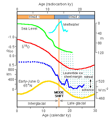
Figure 2. Evidence that northern hemisphere deglaciation at the end of the last ice age was a response to orbital forcing and that the earliest responses were in the northern Atlantic (Nordic Sea) region.

Conceptual Model

The SPECMAP group (Imbrie et al., 1992) proposed that the pattern of lags requires a four state system to explain glacial-interglacial cycles:

• Interglacial
• Preglacial
• Glacial
• Postglacial

Based on the phase relations from the frequency domain analyses, and the nature and magnitude of the changes at critical boundaries (such as the terminations) in the time domain records, Imbrie et al. proposed the following attributes for these four states:

Interglacial

Figure 3. First stage of a generic Milankovitch gl;aciation cycle, according to Imbrie et al. (1992). Symbols for Figures 3-6 are shown below. AA = Antarctic ocean, NOR = Nordic ocean.

During this state, both sea ice and northern hemisphere continental ice caps are at their minimum extents. Deep water is formed in the North Atlantic both by cooling of relatively saline water in the Nordic (Norwegian + Iceland + Greenland) Seas ("Nordic Heat Pump") and by cooling in the Labrador Sea and open Atlantic ("Boreal Heat Pump"). The deep water moves south to the Antarctic, where sea ice is also at a minimum and the westerlies are close to the tip of South America. There the NADW and southern deep water masses mix to create the deep and bottom waters of the Pacific and Indian Oceans. These waters upwell in the North Pacific and Indian Oceans and return to the North Atlantic via surface currents which transport heat and salt to the northern Atlantic source regions where the deep circulation began.

Preglacial

Figure 4. Second stage of a generic Milankovitch glaciation cycle (see Figure 3 caption).

This state is triggered by decreased northern hemisphere radiation, which leads to freshening of the Nordic Seas, thereby terminating the formation of NADW and shutting down the Nordic Heat Pump. The reduction of heat from the north leads to growth in Antarctic sea ice, which pushes the wind field and water masses north. This appears to reduce the rate of overturn of Antarctic waters, which in turn could draw down atmospheric carbon dioxide values.

Glacial

Figure 5. Third stage of a generic Milankovitch glaciation cycle (see Figure 3 caption).

This state results from the continuing growth of the northern ice caps which steer northern hemisphere winds. These produce more convection in the boreal Atlantic, and possibly Pacific (analogous to that occurring in the Labrador Sea today) thereby providing "younger" NAIW and NPIW. The loss of water to the ice caps eventually lowers sea level to the point where ice sheets are grounded on large areas of the continental shelf.

Deglacial

Figure 6. Fourth (final) stage of a generic Milankovitch glaciation cycle (see Figure 3 caption).

As high latitude northern hemisphere radiation increases, the atmosphere and surface waters warm, evaporation increases, and sea ice retreats from the Nordic Seas. The initial retreat of the glaciers modifies the winds to drive warm saline Atlantic water northward. This accelerates glacial melting and provides the buoyancy flux necessary to turn on the Nordic Heat Pump and form NADW, apparently to a greater extent than during full interglacials, thereby transporting heat to Antarctica to accelerate sea ice melting there and enhanced ventilation of the southern deep water, thereby releasing trapped carbon dioxide and setting the stage for a catastrophic collapse of the continental ice sheets.

Multistage Delay-Response Model

Figure 7. Mathematical model of 23 and 41ky responses to radiative forcing at 65 N. Si are linear subsystems (components listed at top of figure) having either delays (d) or time constants (T).

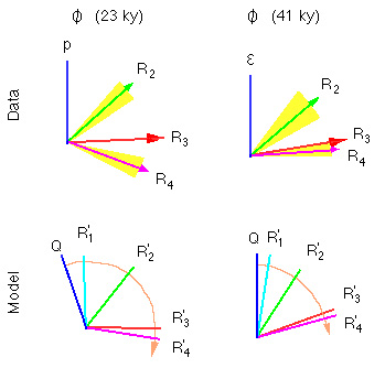
Figure 8. The phase clocks show the goodness of fit between the model of Figure 30-5 and data. Note that R1 is not sampled by the available time series, but is inferred from the time domain relationships.

After iteration, the fit between models and data is reasonable, particularly if the date of maximum 65 N radiation is shifted from mid-June to early June or late May.