where

A periodic signal can be represented by its intensity or amplitude as a function of time:
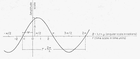
Figure 15-1

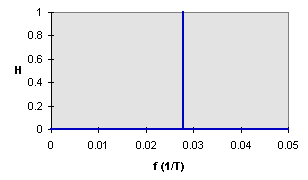
| Time Domain | Frequency Domain |
|---|---|
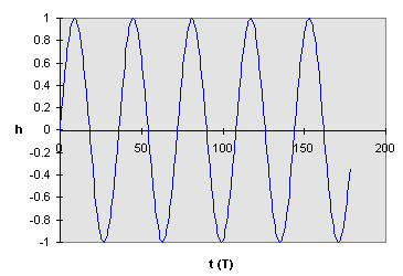 | 
|
Eq 15-1:![]()

(recall that ![]() so the Fourier transform has real and imaginary components).
so the Fourier transform has real and imaginary components).
The original time series can be obtained from the inverse transform:
Eq 15-2:![]()

The transforms can be thought of as weighted averages of waveforms of a given frequency; the forward transform to the frequency domain weighted by the signal amplitude h(t) and the inverse transform to the time domain weighted by the frequency amplitude H(f). In other words, when the signal h has the same frequency as the waveform, the the integral H is large.
If h(t) is real (we are generally considering real signals) then H(f) is generally a complex number. However under this condition H(-f)=H(f)*. (the notation * denotes the complex conjugate). This symmetry means that for real signals there is no unique information in the negative frequencies.
The power of the signal, P, is a measure of its squared amplitude. The power at a frequency f is defined as:
Eq 15-3:![]()

and so the total power in a signal is (fix equation, no (f) on lhs):
Eq 15-4:![]()

Equations 16-1 through 16-4 apply to a continuous function spanning all times. In general though real signals will:
Eq 15-5:![]()
![]()
The quantity 1/![]() is the sampling rate. For any particular sampling interval there
is an frequency f
is the sampling rate. For any particular sampling interval there
is an frequency f![]() called the Nyquist critical frequency:
called the Nyquist critical frequency:
Eq 15-6:![]()
![]()
What is the significance of the critical frequency? There are two related issues.
If the spectrum of h(t) is zero outside of the frequency interval -fc<f<fc, then all spectral information is
obtained if the signal is sampled
at times separated by no more than 1/(2![]() ).
This means that we gain no spectral information by sampling at a rate greater than
the Nyquist frequency.
We can see why by
examining the periodic signal in this figure:
).
This means that we gain no spectral information by sampling at a rate greater than
the Nyquist frequency.
We can see why by
examining the periodic signal in this figure:

Figure 15-3
The period of the signal is 36 time units and so the Nyquist frequency is 1/18 time units. If we sample time unit by time unit, we get a smooth curve. Even if we sample by 18 time units, the Nyquist period, we get (provided we are not exactly in phase with the zero crossings) the highs and the lows so that we still capture the period of the signal. If we sample by 36 time units though, we only get a single value--the signal is constant through time.
Insuring that H(f)=0 beyond the Nyquist frequency is achieved in practice by applying a low pass filter (a filter that lets low frequencies pass the filter, but not high frequency components) to the signal before sampling (as we will see, nature applies a low pass filter through bioturbation in the surface-most sediments).
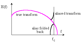
Figure 15-4. The width of the true transform is 2fc; the band from fc to 3fc maps to fc to -fc, the band from 3 fc to 5fc maps to -fc to fc, and so on.)
To understand the nature of the filtering effect of bioturbation consider as an example a core taken in sediments accumulating at 3 cm/ky and sampled at 10 cm intervals. Thus, the sampling interval is 3000 y and so the Nyquist frequency is 1/6000 y.
To model bioturbation, consider
a well mixed box of height h at the sediment surface with material delivered at
rate F and removed as the product of sedimentation rate times
concentration uc![]() . A mass balance can be written:
. A mass balance can be written:
Eq 15-7:![]()

or rewriting in terms of a periodic variation in the delivery of material:
Eq 15-8:![]()
![]()
This differential equation can be solved for some arbitrary initial condition to find that at large times, when initial conditions have decayed, there is a stationary solution:
Eq 15-9:![]()

This equation can be simplified at the limits of high and low frequency. When f is large (the supply of material to the sediment varies at high frequency) it reduces to:
Eq 15-10:![]()
![]()
In this case mixing averages the fluctations in the supply of rain to the sediment. When f is small (the supply to the sediment varies slowly) it reduces to:
Eq 15-11:![]()

In this case the periodic signal is preserved. In other words, low frequency signals are preserved while high frequency ones are not; the system acts as a low pass filter. The boundary between "low" and "high" frequency is effectively f~u/h. For a depth of bioturbation of 2-10 cm in our sample core, this frequency is somewhere between 1/600 y and 1/3000 y. By carefully choosing the sampling interval, little aliasing is possible. (And of course we can also apply a low pass filter to be sure.) Conversely, a limit exists for the highest frequency signal that can be resolved in a core.
Mathematica is a useful tool for solving Eq 15-8 | Download Notebook
The time series analysis of a record consists of a series of computational steps. Depending on the application these might include:
Spectral estimation
If we have N measurements of a parameter h sampled at an interval ![]() then these
occur at times t
then these
occur at times t![]() =k
=k![]() with k=0,...,N-1.
We introduce the notation for the values at these times: h
with k=0,...,N-1.
We introduce the notation for the values at these times: h![]()
![]() h(t
h(t![]() )
From these N measurements we can derive independent information at only N discrete
frequencies--these are normally spaced evenly within the Nyquist limits:
)
From these N measurements we can derive independent information at only N discrete
frequencies--these are normally spaced evenly within the Nyquist limits:
Eq 15-12:![]()
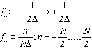
With these conventions the discrete Fourier transform is written:
Eq 15-13:![]()

The power at each of these frequencies is:
Eq 15-14:![]()
![]()
This information can be plotted in the form of a periodiogram:
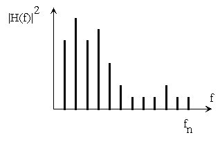
Figure 15-5
Windowing
A common problem is that these estimates are not within the bin implied by the geometry; they actually have a spread several bins wide. A process termed data windowing minimizes this leakage between bins. It involves applying a windowing function to the data before forming the transform:
Eq 15-15:![]()
![]()
Then the power density is given by:
Eq 15-16:![]()

The origin of the leakage between bins arises in the process of taking a portion out of a long time series. Consider this time series h and window function w:
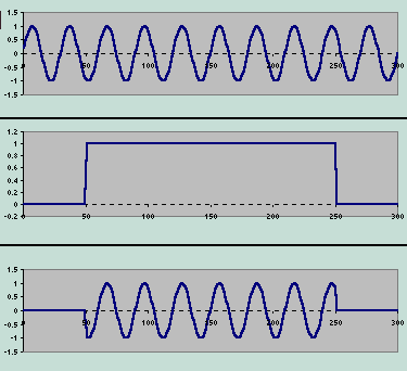 Figure 15-6
Extracting a discrete portion out of the time series h is equivalent to multiplying h by a window function w where w=1 in the region of interest and 0 everywhere else. The convolution theorem say that for two functions h(t) and w(t), if p=wh then P(f)=W(f)H(f). When the discrete transform is taken, the high frequency components associated with the steps in the function w are aliased into the Nyquist interval. The characteristic of a good window is to smoothly turn "on and off", thereby minimizing the introduction of high frequency components into the transform.
Autocorrelation
In performing time series analysis, one can work with autocorrelated records to produce a correlogram. If the Fourier transform of h(t) is H(f), and the autocorrelation function of h(t) is r, then the Fourier transform R(f)=|G(f)|2. For N data points taken from two times series g and h, the correlation as a function of the lag j is:
Eq 15-17:![]()
![]()
Eq 15-18:![]()
![]()
Imagine a periodic function that is shifted progressively to the right:
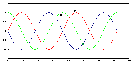
Figure 15-7
As it is shifted the correlation will drop, then rise to the same value when the function has been shifted exactly one cycle:
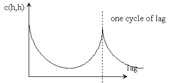
Figure 15-8
Thus the autocorrelation produces a different time series, but with the same spectral components.
Detrending, whitening
There are generally long period and d.c. components that give rise to power in a spectra being concentrated at low frequencies. High pass filters can be applied to remove the d.c. baseline (detrending) and long period, low frequency components (whitening). The effect is to emphasize peaks at intermediate frequency, which no longer sit on the shoulder of a larger low frequency peak.
Thus far we have emphasized frequency characteristics of a time series. Time series analysis also includes consideration of the frequency components within the time domain. These are separated by:
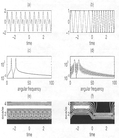
Figure 15-9
chapter on Fourier and Spectral Applications develops background for some basic algorithms
survey of data analysis, including spectral methods
a comprehensive treatment, used for Charlie Eriksen's Data Analysis course
| Oceanography 540 Pages Pages Maintained by Russ McDuff (mcduff@ocean.washington.edu) Copyright (©) 1994-2001 Russell E. McDuff and G. Ross Heath; Copyright Notice Content Last Modified 1/19/2001 | Page Last Built 1/19/2001 |