Lithospheric Subsidence and Sea Level

Topography versus Age

Figure 4-1

If we compare the masses (we should actually consider the weights, but we will take the gravitational acceleration as constant) of the two columns A (at the rift axis) and B (at some arbitrary age), we can derive a relationship for the subsidence, w.

Mass of column A

Eq 4-1:

Mass of column B

Eq 4-2:

where w is the water depth below the ridge, z is the thickness of the lithosphere, and is density. The subscripts w, L and m denote water, lithosphere, and mantle (i.e., asthenopshere), respectively. Equating M and M and rearranging:

Eq 4-3:

The left term is positive, since the lithosphere is cooler and denser than the asthenopshere, and represents the effect of thermal contraction; the second term is negative and represents the effect of replacing denser mantle with lighter seawater as the seafloor subsides.

The specific volume, v, is a state variable v=v(T,P) and so a variation of v can be represented by:

Eq 4-4:

where is the isothermal compressibility and is the volumetric coefficient of thermal expansion. For an unconstrained material (e.g., a material undergoing isostatic adjustment) the pressure does not change when the temperature and volume change, i.e., dP=0, and:

Eq 4-5:

so that

Eq 4-6:

Therefore the change in density associated with thermal contraction can be expressed, using plastic, uncooled mantle as a datum (the M subscript) as:

Eq 4-7:

The temperature distribution in the lithosphere is taken from the conductive boundary layer model for the plate (rewriting the solution in terms of erfc(x)=1-erf(x)):

Eq 4-8:

Substituting equations 4-7 and 4-8 into equation 4-3 and solving for w we find that:

Eq 4-9:

Because the error function complement term in the integral of equation 4-9 approaches zero at the base of the lithosphere, the upper limit of integration can be changed from z to infinity without introducing appreciable error. (This is equivalent to saying T-T approaches zero at the base of the lithosphere, see equation 4-7). With this change of limit and a variable substitution:

Eq 4-10:

equation 4-16 becomes:

Eq 4-11:

The definite integral in equation 4-11 can be evaluated:

Eq 4-12:

so that:

Eq 4-13:

Since the depth to the seafloor is of the form:

Eq 4-14:

the depth-age relationship can be expressed as:

Eq 4-15:

We can make an estimate of w using a value of T of 1350 °C, the thermal conductivity of mantle rock (Lecture 3), and the coefficient of thermal expansion for the mantle:

Eq 4-16:

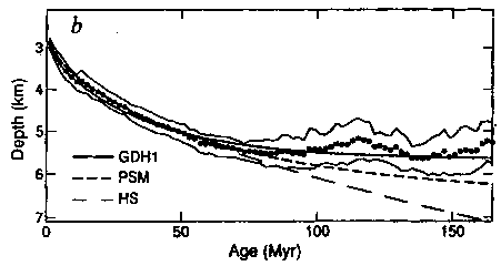
This relationship is apparent in observations as seen in this summary of seafloor topography versus age, from (43)

Figure 4-2. Seafloor topography versus age compared to models of thermal subsidence. HS is the infinite half space model, PSM is the original Parsons Sclater model ((8)), GDH1 is the more recent Stein and Stein ((43)) fit to their complilation of global data.

Variants on Boundary Layer Model

Three refinements to the boundary layer approach have been considered in the literature and applied in variations combinations (see Parsons and Sclater (8) for references):

1. extending the model to two dimensions and explicitly considering the horizontal advection of heat by the plate:

   Eq 4-17:

2. With T(x=0)=T, the heat flux was unbounded at the axis of spreading. Refine the boundary condition at the ridge axis so that heat leaving the axis by conduction and advection matches the heat carried by injected material (i.e., apply a flux condition)

3. Establish a geometry for the model domain such that there is an asymptotic plate thickness and fix the temperature at that lower boundary.

In the past decade, Stein and Stein (43) have undertaken a substantial effort to revisit various aspects of the plate model in order to take full advantage of the data sets that have been obtained since the early Parsons and Sclater work. More information is available at the Seth Stein page. Material properties can be extracted from best fits of improved models (Parsons and Sclater, 8, Stein and Stein (43)):

Fits to Parameters of the Plate Model

	North Pacific (8)	North Atlantic (8)	Global (43)
asymptotic lithospheric thickness (km)	125	128	95
boundary temperature (°C)	1333	1365	1450
thermal expansion coefficient (°C)	3.3 x 10	3.1 x 10	3.1 x 10-5

The agreement is quite satisfying in that each of these three parameters can be related to other observations (the thickness of the lithosphere to seismic studies of upper mantle structure, the boundary temperature to laboratory observations and thermodynamic calculations of melting of mantle rock, the thermal expansion coefficient to studies of physical properties of mantle rock).

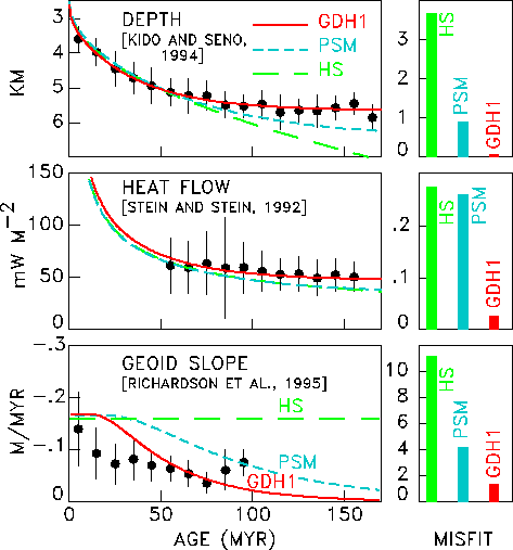
Figure 4-3. Fits by Stein and Stein ((43)) to various models for the thermal behavior of the lithosphere.

Subsidence and Sea Level

The mean age of an ocean basin is inversely related to spreading rate: slower spreding increases the mean age, thus there is more subsidence, and sea level falls.  How much?  The mean subsidence wbar of a basin of width W with spreading rate u is:

Using km as the distance unit and My as the time unit, we can first compute the subsidence for a basin 6000 km wide as a function of spreading rate

and then calculate the change in mean subsidence brought about by a factor of two decrease in spreading rate

This change occurs over a time scale ~100 My so that the rate of change is quite small on human time scales (less than a millimeter per century)

Converted by Mathematica  (October 7, 2002)